Predictive Analytics

Home

The last 25 years have seen a great deal of progress in the use of data to analyze and forecast the behavior of complicated systems.

In response to these developments, the two main credentialing bodies for actuaries, the Society of Actuaries and the Casualty Actuarial Society made extensive revisions to their exam syllabi in 2018.

The Society of Actuaries now have two exams covering predictive analytics. The first of these requires candidates to produce a data-driven solution to a complicated business problem using the R and RStudio software.

One of the main reference texts is An Introduction to Statistical Learning, with Applications in R by Stanford authors James, Witten, Hastie, and Tibshirani. The first edition, which I used in courses I taught at Stonehill College, is available as a free download, with your choice of R or Python code examples.

You can find a sample exam with solutions here.

It is my intent to make use of these 21st century techniques to provide improved financial analytics and forecasting for the East Greenwich School Department.

Forecasts versus Projections

It is important to understand the difference between forecasts and projections, both of which are used to gain insight into the future behavior of systems.

Projections	Forecasts
Make as many strong assumptions as necessary to rule out all but one outcome	Try to avoid strong assumptions
Usually no underlying mathematical model	Usually has an underlying mathematical model
Provides only a single point estimate of the quantity of interest	Provides a probability distribution for the quantity of interest (Bayesian)
Provides no information on the variability of the estimate	Provides variability estimates
Cannot easily validate with historical data	Can validate with historical data (in fact it's considered mandatory)
Cannot easily handle situations with multiple parameters	Can handle multiple parameters with joint distributions
Usually requires nothing beyond high school math and a spreadsheet	Requires a solid mathematical foundation including multivariable calculus and specialized software (MCMC)

Step 1: The Data Generating Process for the School Appropriation

The modeling process usually starts by defining a process that generates data similar to what we observe. This is characteristic of a Bayesian approach and affords an opportunity to incorporate domain knowledge into the model that might not be reflected in a generic model.

In the case of the local tax appropriation, we have two important constraints on its size:

Maintenance of Effort requires that the appropriation be at least as large as that of the prior year.
The 4% Levy Cap limits the new appropriation to no more than 4% above the porevious year. There is some ambiguity about whether this applies separately to the town and school department appropriations, but for simplicity we will assume the school appropriation cannot increase by more than 4% in a year.

It's good to start with a simple model, and one obvious choice is a model having the expected value of each successive appropriation equal to a multiple of the previous one, with the multiplication factor chosen to be between 1.00 and 1.04. In fact, this is a well known classical time series model of the ARIMA (Autoregressive Integerated Moving Average) type, designated AR(1).

To complete the model, we add some random noise in the form of Gaussian error terms each with expected value zero and a common standard deviation.

If \(y_i\) is the appropriation at time \(i,\) \(e_i\) is a Normal \((0,\sigma)\) random variable, and \(\alpha\) is a random variable that takes values between zero and one, then \[y_{i+1} = y_{i}\cdot(1+\alpha\cdot(0.04)) + e_i\quad i=1,2,\ldots,n\] is a modified AR(1) model with a built-in restriction that the multiplier of \(y_i\) has to be between 1.00 and 1.04.

Results of the Data Generating Process for the School Appropriation

core coverage

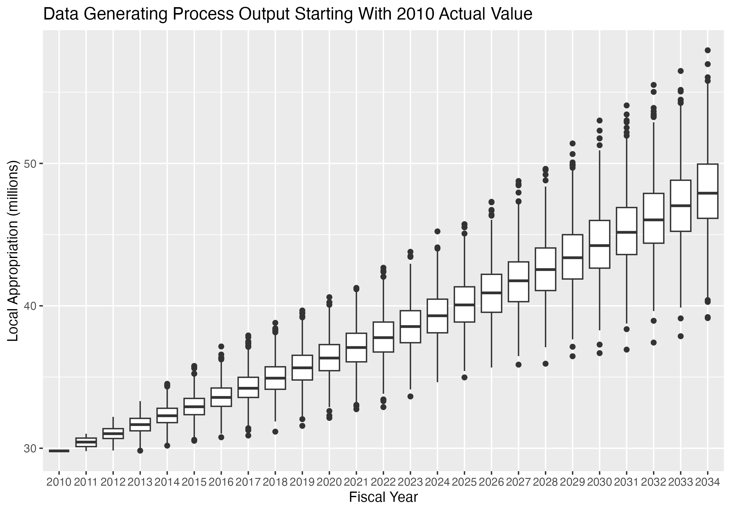
If we generate pairs of \(\alpha\) and \(e\) values, and supply an initial value for \(y_1\) equal to the 2010 appropriation, the result is called the prior predictive distribution.

It represents the distribution of values that results from the prior distribution of the parameters.

Because the AR(1) model requires a single initial value as a starting point, we supply the 2010 appropriation as the starting value.

That is the only data point used to produce this graphic. All other features are produced by the data generating process and the priors.

Results of the Data Generating Process with Actual School Appropriation Values Superimposed

core coverage

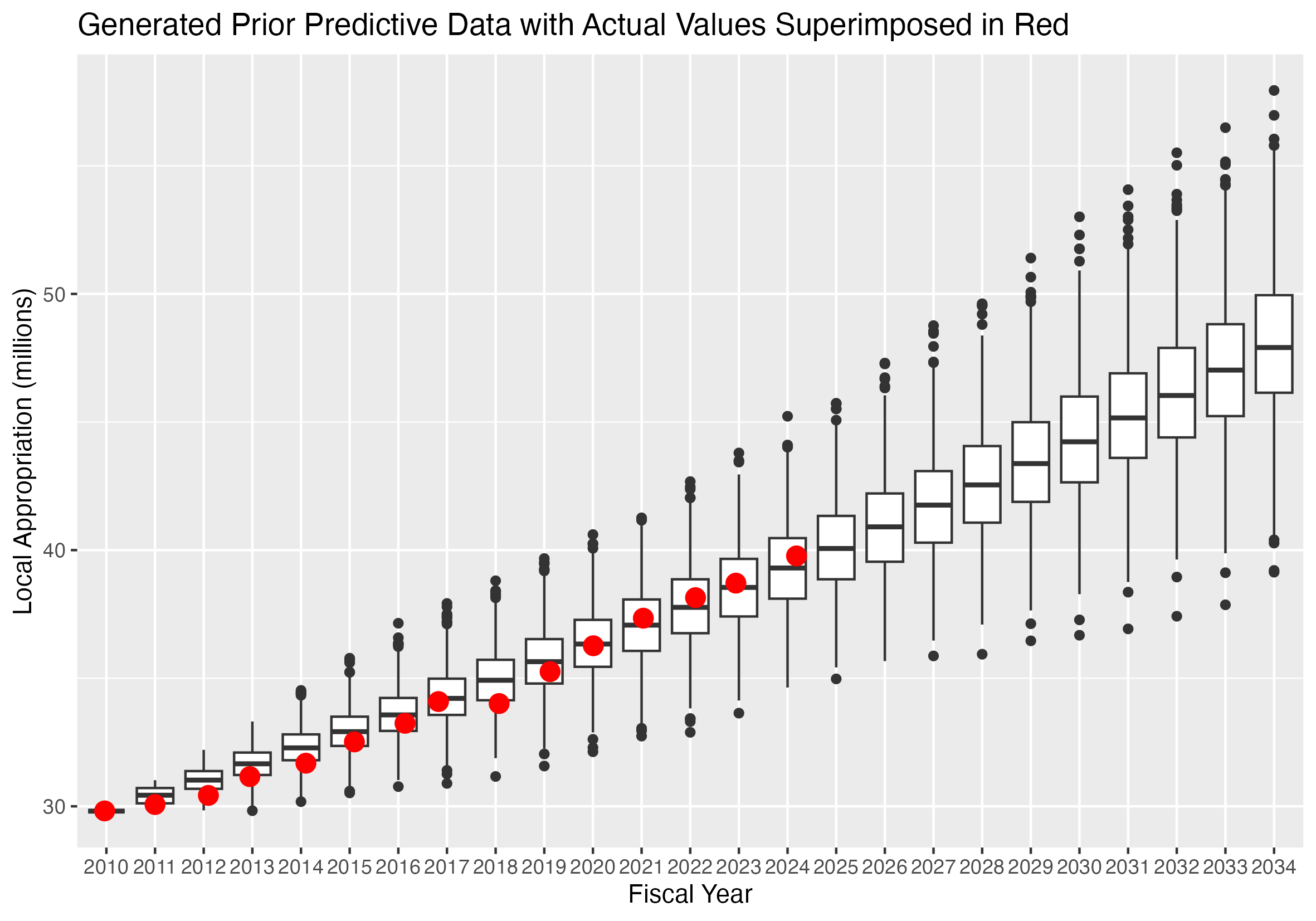
This graph shows the prior predictive distribution with the observed values superimposed as red dots.

The prior predictive data was generated from a single data value, the 2010 appropriation.

School Appropriation - Posterior Predictive 5 Year Forecast 2015-2019

core coverage

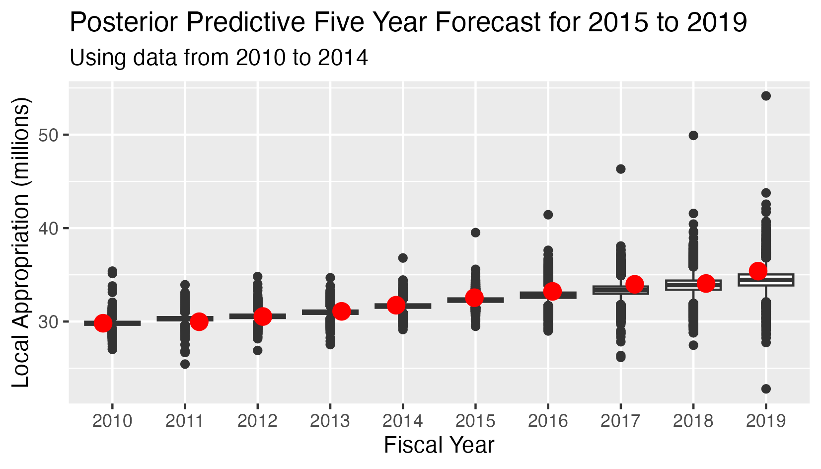
The posterior predictive distribution uses a Markov Chain Monte Carlo procedure to combine observed data points and priors.

Instead of a single observed data point, this analysis has:

Five observed values for the appropriations in years 2010-2014
Five conditional predicted distributions for the appropriations in years 2015-2019.
The red dots indicate the observed value in all cases.
The Mean Square Error (MSE) for the five predicted values is 0.296

The posterior predictive distribution is the joint conditional distribution of the appropriations for 2015-2019, given the observed values for 2010-2014 and the prior distributions of the parameters.

In the probabilistic model setting, the optimal point forecasts for 2015-2019 are the expected values of the conditional distribution of the appropriations given the priors and the observed values for 2010-2014.

School Appropriation - Posterior Predictive 5 Year Forecast 2016-2020

core coverage

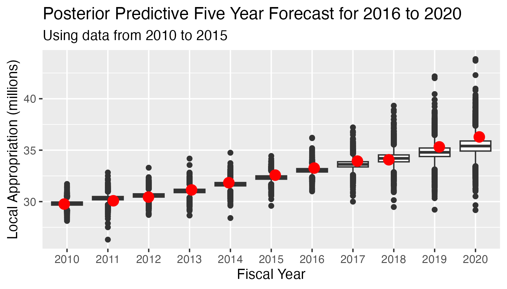
This analysis has:

Six observed values for the appropriations in years 2010-2015
Five conditional predicted distributions for the appropriations in years 2016-2020.
The red dots indicate the observed value in all cases.
The Mean Square Error (MSE) for the five predicted values is 0.267

The posterior predictive distribution is the joint conditional distribution of the appropriations for 2016-2020, given the observed values for 2010-2015 and the posterior distributions of the parameters.

School Appropriation - Posterior Predictive 5 Year Forecast 2017-2021

core coverage

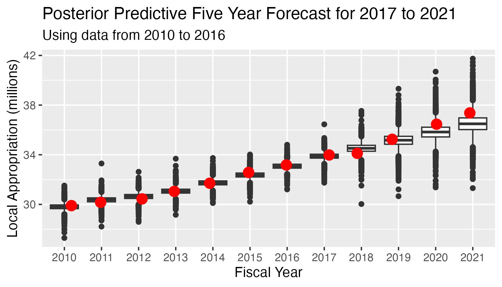
This analysis has:

Seven observed values for the appropriations in years 2010-2015
Five conditional predicted distributions for the appropriations in years 2016-2020.
The red dots indicate the observed value in all cases.
The Mean Square Error (MSE) for the five predicted values is 0.282

School Appropriation - Posterior Predictive 5 Year Forecast 2018-2022

core coverage

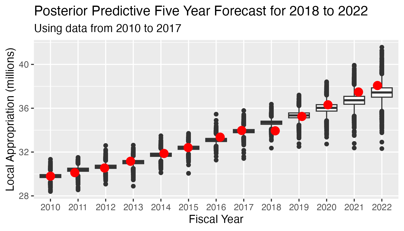
This analysis has:

Eight observed values for the appropriations in years 2010-2017
Five conditional predicted distributions for the appropriations in years 2018-2022.
The red dots indicate the observed value in all cases.
The Mean Square Error (MSE) for the five predicted values is 0.297

School Appropriation - Posterior Predictive 5 Year Forecast 2019-2023

core coverage

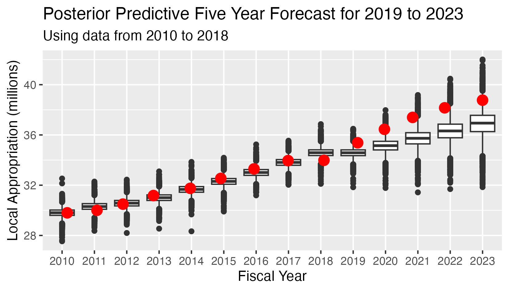
This analysis has:

Nine observed values for the appropriations in years 2010-2018
Five conditional predicted distributions for the appropriations in years 2019-2023.
The red dots indicate the observed value in all cases.
The Mean Square Error (MSE) for the five predicted values is 2.25

In 2018 the school department was level-funded, so this data point is an outlier. Because the AR(1) model gives considerable weight to the most recent data point, the predicted values are considerably lower than they normally would be. This accounts for the high Mean Square Error.

School Appropriation - Posterior Predictive 5 Year Forecast 2020-2024

core coverage

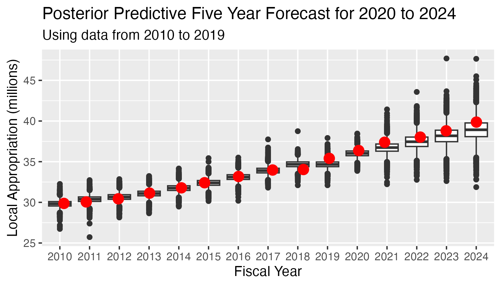
This analysis has:

Ten observed values for the appropriations in years 2010-2019
Five conditional predicted distributions for the appropriations in years 2020-2024.
The red dots indicate the observed value in all cases.
The Mean Square Error (MSE) for the five predicted values is 0.454

This time the last data point lies more or less on the trend line, so the Mean Square Error decreases substantially. It will decrease further as the 2018 anomaly recedes into the past.

Posterior Predictive 2022 School Appropriation

core coverage

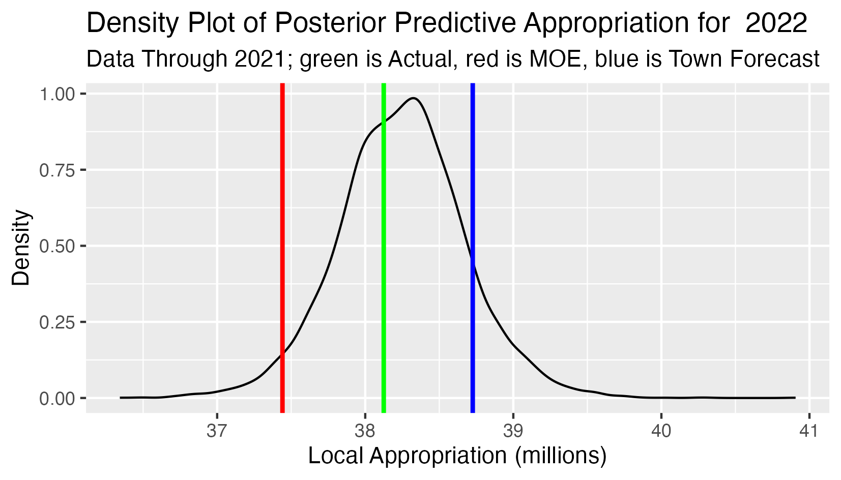
This analysis has:

All observed appropriations 2010-2021 as input data.
The black curve is the density function of the predictive distribution of the 2022 school appropriation.
The green line is the actual 2022 school approppriation (forecasting one year ahead).
The red line is the lower limit defined by the Maintenance of Effort requirement (the 2021 school appropriation).
The blue line is the school appropriation projection from the town forecast.

Posterior Predictive 2023 School Appropriation

core coverage

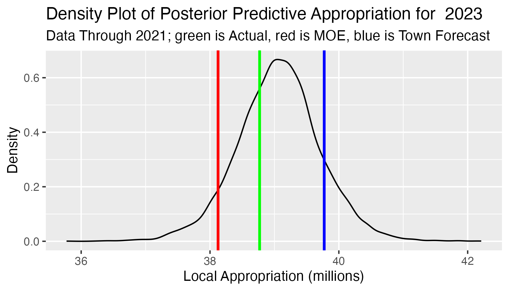
This analysis has:

All observed appropriations 2010-2021 as input data.
The black curve is the density function of the predictive distribution of the 2023 school appropriation.
The green line is the actual 2023 school approppriation (forecasting two years ahead).
The red line is the lower limit defined by the Maintenance of Effort requirement (the 2022 school appropriation).
The blue line is the school appropriation projection from the town forecast.

Posterior Predictive 2024 School Appropriation

core coverage

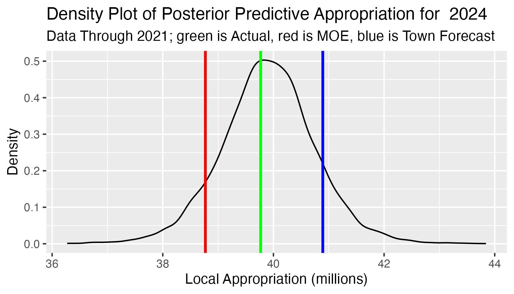
This analysis has:

All observed appropriations 2010-2021 as input data.
The black curve is the density function of the predictive distribution of the 2024 school appropriation.
The green line is the actual 2024 school approppriation (forecasting three years ahead).
The red line is the lower limit defined by the Maintenance of Effort requirement (the 2023 school appropriation).
The blue line is the school appropriation projection from the town forecast.